Last August, we covered some of the highest-level concepts about GeoAI in an attempt to demystify it. If you haven’t already, I recommend reading that article before continuing. If you already have, welcome to part two of the series! We’re happy to have you.
Today, we’re going to be digging into what goes on “under the hood” of GeoAI. To get us started, we’re going to focus on traditional machine learning methods. These will be fundamental to our ability to apply advanced deep learning to geospatial data.
At the core of any machine learning project is a model, which is trained to detect patterns within the data. There are many different types of models, each with varying complexity, strengths, and weaknesses. To get us started, we’ll focus on the simplest of them all: the Decision Tree.
Decision Trees
A decision tree essentially works just like a flow chart; it asks a question and provides a path based on the answer to that question. At the end of each branch on this tree, you end up with leaves, which represent a prediction based on the path it took to get there. Take, for example, this image depicting a decision tree about whether or not to accept a new job offer:
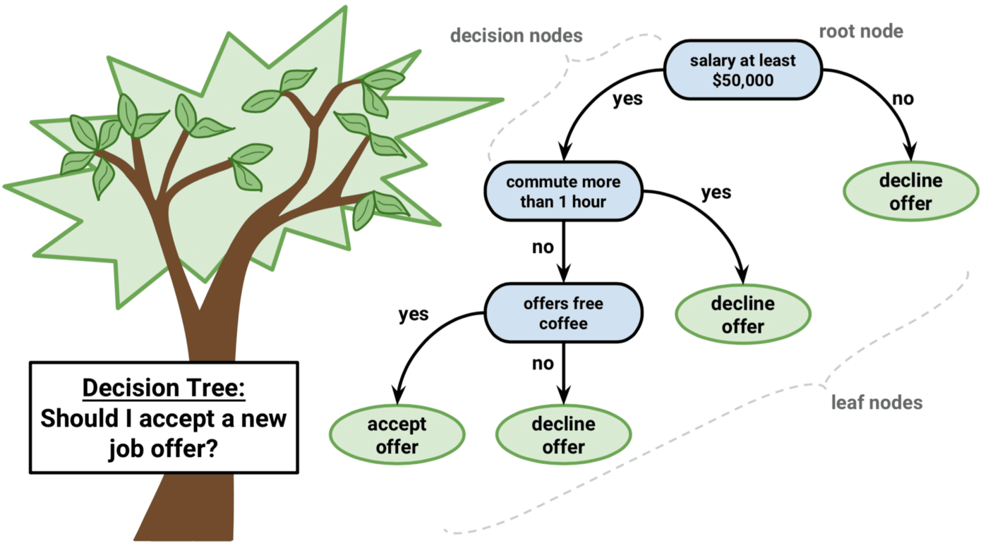
This tree has a total of four leaves, three of which result in the same outcome (or prediction). Now of course, there wouldn’t be much point in machine learning if you had to make all of the decision nodes for it. After all, that’s why you’re training it! The good news is that when you are setting up your own decision tree learning project, the machine determines the decision nodes to get to the most accurate predictions — you do however need to provide the parameters (or constraints) for it to operate under.
Training Your Dataset
Once you’ve initialized your model with its constraints, the next step is to “fit” it with training data. This data is your control set — it contains information in the same format you’d like your model to create predictions for, but you already know the answers. By giving the model both the data and the correct value, you are teaching the model how to make its predictions.
Since you’re in control,- you might be tempted to just open the floodgates here and tell it to make a decision tree with hundreds or thousands of leaves. After all, the more complex the tree is, the more likely the model has a precise branch for any variable it encounters in the data, right?
Not quite, as it turns out. While a decision tree with an excessive amount of leaves can make almost perfect predictions on the data it was trained on, it will often make far worse predictions when it analyzes a totally different set of data. The reason for this is a phenomenon called overfitting, which means that the model is essentially too rigid in its thinking.
It was tasked with creating decision nodes leading to 100 different leaves on the training data, and the training data contained exactly 100 different outcomes. The good news is that the model detected exactly which combination of factors resulted in each of these outcomes — the bad news is that now it’s fairly sure that the only way to get to each of those outcomes is by the exact set of circumstances that got it there in the training data.
As a result, it’s going to be really confused when you aim it at data that combines these attributes in a different way.
The opposite of overfitting is, underfitting, or when the model is too loose in its thinking and overlooks key factors. This can happen when the model is trying to the decisions simple. An example of this would be a very simple two-leaf decision tree that attempts to predict the average price of houses based on a single factor: if the house has 2 or more bedrooms, the price is $X, otherwise, the price is $Y.
You can already see how this would be far too simple of a way to predict the price of the house – after all, there are so many other factors to consider.
Testing Your Dataset
Once you have fit your data into your model, the next step is to test how well it learned to make predictions. To do this, you’ll need a separate set of data from your training data. You’ll also need to have the answers for this data, but the difference is that you won’t give those answers to your model like you did when you were fitting it.
You run the model on your validation data, then compare its predictions to the answers that you already have to determine how close they are.
Comparing the predictions to the correct answers results in a Mean Absolute Error, or MAE. The MAE is a measure of how close the model was able to get to the real answer with its predictions.
Generally speaking, a lower MAE is better. In order to get good predictions from your models, you will need to test many different combinations of parameters and assess the resulting MAE of each.
Decision trees are always going to attempt to find the correct balance between underfitting and overfitting. Luckily, there are other, more advanced models that attempt to alleviate this problem.
Random Forest, for example, creates many different decision trees and uses the average result of each tree for its predictions. This extra complexity can smooth out predictions and often result in a lower MAE than a single-tree model.

Prepping Data
There are many other types of models, but for now let’s move on to what you’ll need to do to prepare the data for being used with the model you’ve chosen. Real world data often isn’t perfect — some information might be missing or otherwise invalid in your chosen base data. Machine learning doesn’t do well with missing data, so you’ll need to sanitize your data before you use it for training or run predictions against it.
You can sanitize your data by dropping columns containing any missing values, but this could also drop a lot of valuable information as well. You can instead drop any rows that contain missing values, but this can reduce the accuracy of your model by resulting in a smaller set of training data.
Rather than dropping the values, you can instead impute them. Imputing a value means filling in the missing values with a valid option. This value could, for example, be the average of all other values in the same column. This won’t be exactly correct, of course, but it is preferable to dropping the entire column or row due to all of the other data that would be lost if you did that.
Because machine learning does best with numerical data, another type of pre-processing you’ll need to perform on your data is to remove categorical variables. A categorical variable is something that takes a limited number of values, such as a feature type attribute with coded domain values limiting the selection to one of 5 possible feature types. To remove these categorical variables, we have a few options:
Drop the Categorical Data
Dropping the data is the easiest approach, but it suffers from the same downside as removing a column or row in the event of missing data. You’re going to lose a lot of potentially important information.
Ordinal Encode
Ordinal encode the categorical data by assigning each unique value to a different integer. Ordinal encoding data works well if the categorical data has an implied or direct ranking to the values (i.e. an attribute that contains values of “Low”, “Medium”, and “High” can be ordinal encoded to 0, 1, and 2).
One-Hot Encode
One-hot encoding is when a new column is created for each possible value in the data, and a numerical value is assigned based on the original value. It does not assume an ordering of the categories, so it can work well in the event that values are not distinctly “less” or “more” than each other. One-hot encoding should be avoided in the event that a categorical variable has a plethora of possible values though, as it can negatively affect the performance of the model.

By taking the time to plan out which model to use and sanitizing your data ahead of run time, you can ensure that you get the kind of results you are looking for with machine learning.
That’s it for this lesson on GeoAI and you! What did you think? What do you want to hear about next? Let us know on Twitter or LinkedIn. If you have a project that you think could benefit from GeoAI, contact us, and we’ll be happy to talk it over with you!